How to remove duplicate or empty rows in Google Sheets

Duplicate rows or empty rows can often be found in Google Sheets, and they can create clutter and hinder data analysis. This may occur when data is accidentally copied or imported multiple times, while empty rows may result from removing things and forgetting you did so, for example!

The good news is that removing these unwanted rows is a straightforward process that requires just a few clicks. Today, I will guide you through the steps to remove duplicate or empty rows in your Google Sheet, helping you clean up your data and improve its organization. Let’s get started!

Method 1: Data Cleanup

Start by clicking on the top leftmost rectangle that connects the row lettering and column numbering. This rectangle acts as a select all button, allowing you to select all the cells in your sheet. you’ve done this, go to the top of the screen and click on “Data”. Then, scroll down and select “Data cleanup”. This will open a dialog box with three options: Cleanup suggestions, Remove duplicates, and Trim whitespace. Obviously, we’ll want to choose “Remove duplicates”.

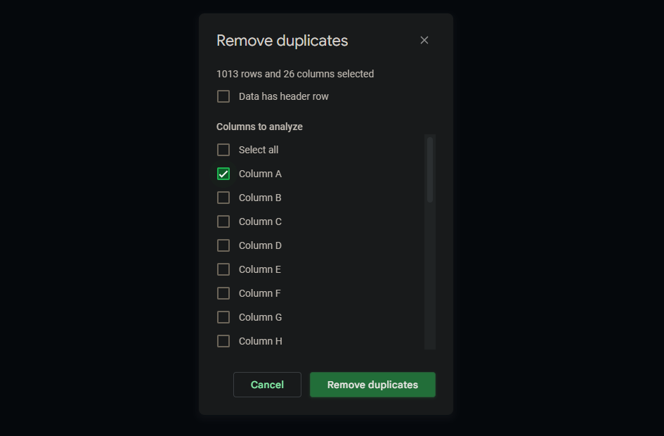
In the dialog box that appears, uncheck the ‘Select all’ button to deselect all columns. Then, re-select only the columns you want to clean up duplicates from. If you have duplicates across the entire sheet, you may want to keep the select all option checked. Finally, click the green “Remove duplicates” button and watch as the magic happens! Instantly, all the empty rows and duplicate data will disappear.

Method 2: Creating a Filter view

If you have empty rows instead of just multiple copies of data, there are other ways to remove them too. The second method for achieving this is by altering your data to separate the rows that have something in them from those that do not. Because you may not want to permanently change the ordering of your data, I recommend a “Filter view”, which is like a temporary version of a filter that can be toggled on and off and is only seen by you.

To use it, go up to Data > Filter views > Create new Filter view. You’ll notice a drastic change in the coloring and style of your spreadsheet with the rows and column labels turning dark grey instead of white, and a new bar above that showing the filter name and range as well as a cogwheel and close out button to turn it off. If you’re just using this view to remove empty rows that were between rows with data, there’s no need to name it since you won’t be keeping it. Also, don’t mind the inverted colors of my screenshots, I’m using a dark mode extension for Chrome – sorry about that!

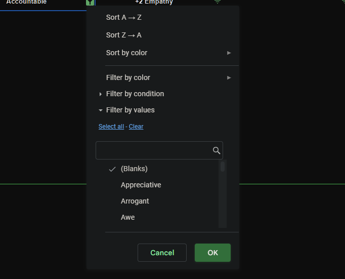
Hover over the filter icon your header text displays and choose the ‘Clear’ button, followed by checking the ‘(Blanks)’ option before hitting the green ‘OK’. After that, you’ll see all of the blank rows clumped together, and all you need to do from that point is highlight and delete them as shown below.

There are other methods for deleting your empty rows in a Google Sheet too, such as sorting the data to clump them together before deleting them or using an add-on like Power Tools, but we won’t cover those today as what we’ve discussed should be plenty sufficient for your needs. Remember to retain the ordering of your data if that’s important to you, even while performing a cleanup. I hope this helps!