How to use the VLOOKUP function in Google Sheets to find things in a table or range by row

Google Sheets is powerful. It’s not as powerful in some ways as Microsoft Excel has become over the past four decades, but it’s stuffed full of functions – Google’s name for formulas – and these can be used to turn the spreadsheet service into a powerhouse for data organization and analysis.

Today, I’m going to help you gain a basic understanding of how the ‘VLOOKUP’ function works so you can use it to find known information in your Sheet and search for related info by row. Essentially, it’s a vertical lookup that takes a key or first column of a range and returns the value or values in specified cells of rows found.

Vertical lookup searches down the first column of a range for a key and returns the value of a specified cell in the row found.

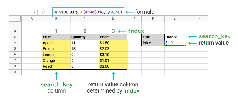
When you enter to VLOOKUP function into any cell as "=vlookup(" Sheets will ask for four criteria with a popup window. First and as previously mentioned the search ‘Key’. Let’s say, for example, that you want to enter a list of fruits and vegetables as ‘keys’ into the first column of your table.

VLOOKUP(search_key, range, index, [is_sorted])

Here’s how the VLOOKUP function is laid out

The second criteria is the range that you want Sheets to consider for the search. For now, we’re going to use the entire table as a range, or at least all of the data in the table. So, you’ll choose the first cell and the last cell as the range.

The third criteria is the index or the column number that you want the formula to use or focus on. Using the example above that Google has provided on its help page, let’s tell Sheets to focus on the quantity column of the table so we can determine how many of each fruit or vegetable exist. In order to determine the index number, count over to how many columns from the left the quantity column is. Google has it placed as the third column, but if your Sheet has keys in the first column, it may make sense to place your quantity in the second column instead.

Lastly, the ‘is sorted’ piece of the formula simply asks you whether or not your keys or the first column in your table (our fruits and vegetable names) is sorted. Google Sheets will try to find as close a match as it can if it can’t find an exact match based on how you set this up, but in most cases, it’s not even necessary!

Once you’ve plugged each piece of the puzzle in, let’s say on a second tab of the sheet, you can turn your keys into a dropdown list and instantly get the quantity and or price among other things of each fruit or vegetable as each will dynamically change once you use VLOOKUP.

Functions aren’t exciting for many people, but once you have an interesting set of data you want to analyze and extract vital info from in order to make important decisions, they can be lifesavers. I’m the type of person who actually really loves this kind of stuff though.

What I’m really interested in, however, is seeing how you and your organization are utilizing the VLOOKUP function in your day-to-day workflow. Let me know in the comments below if you’re using it to sort through students and their test scores, inventory items, and their details, or something else entirely.