How to find and highlight duplicates in Google Sheets

Google Sheets includes an option to find and remove duplicates, but it doesn’t give you a chance to review these duplicates before deciding whether they should be removed or not. Thankfully there is a workaround for this using conditional formatting and a handy formula that highlights the duplicates instead, leaving the rest up to you.

Setting up your conditional formatting formula

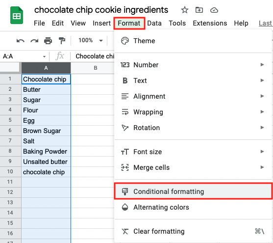
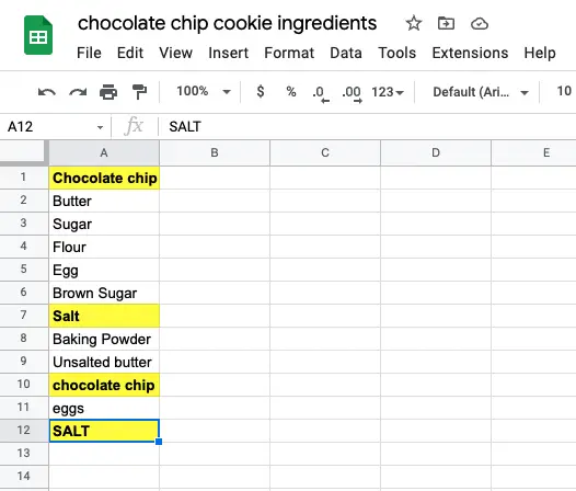
To set up your conditional formatting formula, open the spreadsheet that contains the data you want to work on, and select the cells where you want to find duplicates. In the example below, I am selecting a column of ingredients needed to bake chocolate chip cookies.

Once you have made your selection, click on Format > Conditional Formatting from the Google Sheets application menu.

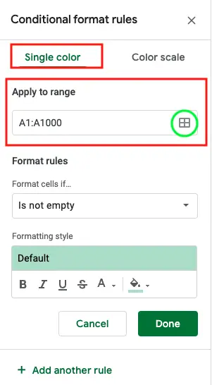
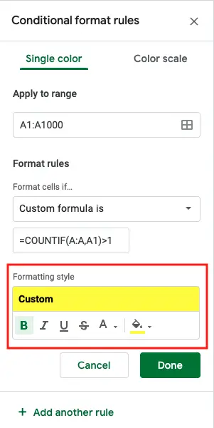
A Conditional format rules panel will open to the right of the spreadsheet. Select the Single color tab on this sidebar, and confirm the range in the “Apply to range” field matches your selected cells. You may edit your range if needed at this point by clicking on the icon that resembles a table and then adjust your selection.

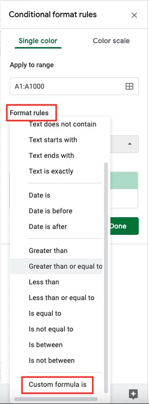
In the “Format rules” section, click on the drop-down and select “Custom formula is“.

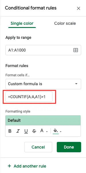
Enter the below custom formula and make the below adjustments:

=COUNTIF(RANGE,CRITERIA)>1

• RANGE: Enter the column range that you previously selected. For simplicity, we would suggest that you use a column range rather than a range of cells. It is much easier to type in A:A to denote all of column A, rather than $A$1:$A$1000 to denote all of the cells. In this example, since I selected Row A, I am going with A:A. If I had selected column B, then I would go with B:B, and so on.
• CRITERIA: Enter the first cell within that selected column that includes data. In my example, the first cell with data is A1, so that is what I will use for my criteria.

Finally, adjust the formatting style to your liking. In my example, Sheets defaulted to highlighting my conditional formatting in green. If I wanted to change this to be in bold and highlighted in yellow instead, then this is where I would make these changes.

Finally, click Done to save your formula and watch as your data now adjusts to show you duplicate values with your custom formatting.

I just want the steps!

1. Open the spreadsheet

2. Select the cells where you want to find duplicates

3. Click on Format > Conditional Formatting

4. Select the Single color tab on this sidebar, and confirm the range in the “Apply to range” field matches your selected cells

5. In the “Format rules” section, click on the drop-down and select “Custom formula is“

6. Enter the below custom formula =COUNTIF(RANGE,CRITERIA)>1 where RANGE is the column of the values you selected and CRITERIA is the first cell with data.

7. Adjust the formatting style to your liking

8. Click Done

Limitations of using this method

As you can probably see in the screenshot above, the formula failed to catch duplicates that are not an exact match, such as plurals. It did, however, catch an all-caps version of the same word. There are more complicated formulas you can use to drill down and get more specific results, but for the purposes of this guide, we are using the simplest and quickest solution.

You can edit and delete this conditional formatting as needed, and although not perfect, it does beat the all-or-nothing solution that Google Sheet currently provides.